

Software manual
ChipScan-ESA 3.1
Notice No part of this manual may be reproduced in any form or by any means (including electronic storage and retrieval or translation into a foreign language) without prior agreement and written consent from Langer EMV-Technik GmbH. The management of Langer EMV-Technik GmbH assumes no liability for damages which may result from the use of this printed information.
1. System requirements and installation
1.1. System requirements
Your computer system should have at least the following properties.
- 1 GB HD space
- CD drive for installation of ChipScan-ESA
- Windows ® XP/Vista/7 (latest service packs)
- Monitor with a display resolution of 1280x1024
- Free USB port for USB dongle
- Spectrum analyzer1 (for trace acquisition only)
The minimum memory requirements strongly depend on the number and the size of the loaded spectrum analyzer traces, whereas the minimum CPU and GPU requirements strongly depend on the number and size of displayed traces. Keep in mind that the number of displayed traces is normally not higher then 10. Displaying up to 1000 or more traces is possible but not really useful for analysis.
Because of these circumstances we just provide a recommended setup for RAM, CPU and GPU. This setup is able to load 10,000 traces each having 1,000 data points and to display about 1,000 of them without any latency.
- 2 GB of RAM
- CPU Intel Core i5 2 GHz
- GPU AMD Radeon 7750
1.2. Installation
- Insert the ChipScan-ESA CD into your CD-ROM drive.
- Change to the directory ChipScan-ESA on the CD.
- Double click ChipScan-ESA.exe.
- Please read the license agreement carefully. If you accept it, you can go on.
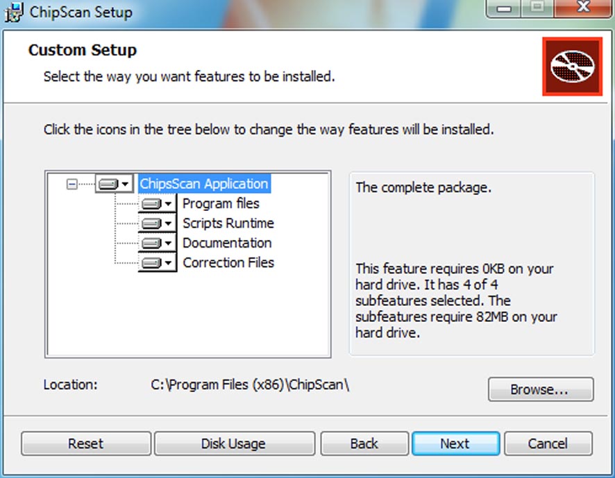
- Select the location where ChipScan-ESA will be installed.
- Finish installation.
- Make sure to plug the USB dongle into a free USB port before executing ChipScan- ESA.
2. Getting started
2.1. Quick introduction into ChipScan-ESA
For users who want to get started immediately here is a quick introduction to ChipScan-ESA. The example data file used in this tutorial can be found in the directory examples in your ChipScan-ESA distribution.
Start ChipScan-ESA by executing it from the Windows® Start menu. ChipScan-ESA will start up with the main window entitled ChipScan-ESA.
The main window allows the viewing of four different dock windows: the visualization which is always visible, the trace manager, the spectrum analyzer manager and the log. If you closed any of the latter windows you can make them visible by selecting the appropriate menu item in the Window menu.
2.2. Viewing spectrum analyzer traces
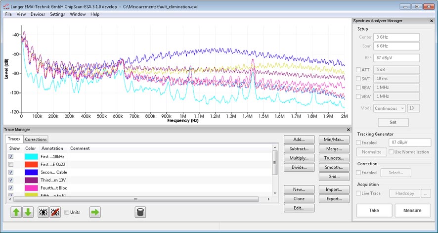
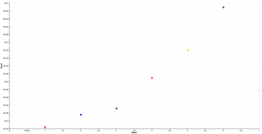
To open a spectrum analyzer traces file select Open... in the File menu. Navigate in the file dialog to the directory where the example data files are located and mark the desired file with a single (left) mouse click. Pressing the Open button opens the file.With the default dock window settings you see the visualization displaying the traces in the center, the spectrum analyzer manager on the right next to it and the trace manager on the bottom (see fig 2.1 ). The spectrum analyzer traces are shown in a Cartesian coordinate system. You can center a point of interest in the traces by moving the mouse while holding down the left mouse key over the visualization. You can zoom in/out of the traces by spinning the scroll wheel. While spinning you may also hold down the Shift or the Ctrl key to zoom along the x- or y-axis only. Moving the mouse pointer over a data point of a trace will display the specific values for x/y-axis including the unit. To recover the full view range of all visible traces press Ctrl+Z or select Zoom Fit in the View menu.
2.3. Manipulating of spectrum analyzer traces
All manipulating actions on traces are made via the trace manager. You can either manipulate the properties of a trace like the visibility, color, etc. or alter the data of a trace itself. In the following we will give only a short explanation of the most used actions. For a more detailed description of all available actions see section 3.4. You can show or hide a specific trace by selecting or deselecting the box in the Show column. To show or hide multiple traces you first highlight the appropriate lines in the trace manager, for example by holding down the Ctrl key and selecting all desired lines one by one. Pressing  afterwards will add or remove the traces from the visualization. You may also change the color of a trace by selecting the rectangular colored field in the Color column and choosing a different color in the subsequent color dialog. To permanently delete any number of traces from the trace manager select the specific lines and press
  .
.
2.4. Acquiring spectrum analyzer traces
To acquire spectrum analyzer traces using ChipScan-ESA it is required that you connect a spectrum analyzer to your PC.1 Make sure it is properly connected. Furthermore, to eliminate any connection problems you may verify your setup with a software provided by your spectrum analyzer manufacturer.
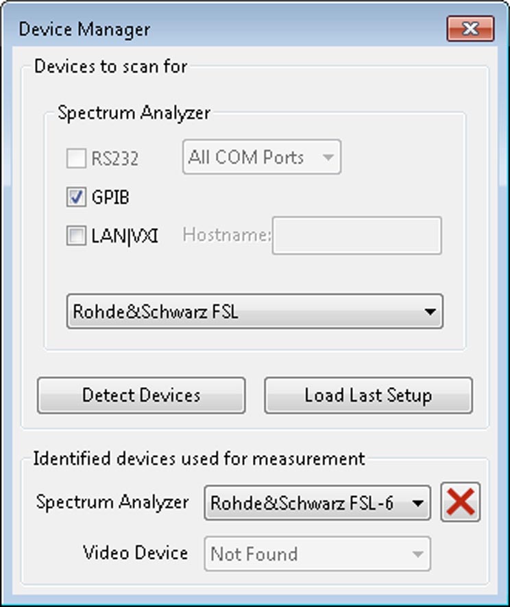
Acquisition of traces is handled via the spectrum analyzer manager. Before using it ChipScan-ESA must detect a spectrum analyzer that is connected to your PC. To do so select Device Manager from the Devices menu. In the subsequent device managerdialog (see fig 2.2) select the interface your spectrum analyzer is connected to and press the Detect Devices button. All connected devices, which have been automatically identified, will be shown in the Identified devices used for measurement section of the dialog. Make sure to select your connected spectrum analyzer from the list of identified devices. If your spectrum analyzer could not be automatically identified please redo the afore mentioned connection test. If it does not succeed please see section 4 for a detailed description of the device manager and its capabilities before contacting our support.
After identifying the connected spectrum analyzer you can change all important properties like frequency range, reference level, etc. of the spectrum analyzer via the spectrum analyzer manager. To finally set the properties press the Set button. Thiswill transfer all settings to the spectrum analyzer. If your spectrum analyzer includes a supported tracking generator you may configure it, too. When finished you can acquire a trace by pressing the Measure or Take button. The trace will be shown in thevisualization and an additional appropriate line containing the trace properties will appear in the trace manager.
2.5. Exporting data and images
Beside saving of acquired spectrum analyzer traces you can also export the trace data. This is especially important for further analysis with statistical software like R or Matlab. To do so select Export data... from the File menu and specify the file inthe subsequent file dialog where the data should be saved to. The resulting file (.csv) will contain a comma separated value list of all traces currently available in the data manager.
Furthermore you may want to export the image of the current visualization for purposes like presentation or documentation. To do so select Export image... from the File menu and a file dialog will open. There select a filename and an image type to finallysave the image in a file.
3. Graphical user interface
The layout of the graphical user interface of ChipScan-ESA is partly configurable to meet your demands during different tasks. It uses a dock window system, which allows to rearrange some windows of the graphical user interface within the main window.Apart from the visualization there are three main dock windows, the spectrum analyzer manager, the trace manager and the log. The visibility of each window can be set in the Window menu by selecting the appropriate entry.
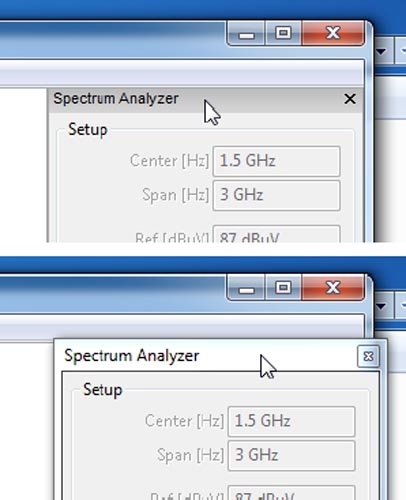
To undock any windows move the mouse pointer over the upper frame of a docked window, press and hold down the left mouse button and drag the window to the desired position (see fig . 3.1). ChipScan-ESA will rear-range the main window in order to fit everything into it,thus all other docked windows will fill out the available space automatically. Using the undock option can bevery helpful to gain more space for the visualization on small monitors.
Additionally you can hide any docked or undocked windows by pressing the x symbol in the upper window frame. This option is especially useful if for example you evaluate your measured traces. During this task you would not need the spectrum analyzer manager at all. To show any hidden dock windows you need to select the appropriate entry from the Window menu.
You can also dock all undocked windows but the log window back to the main window. Be aware that the possible dock position varies from window to window. The spectrum analyzer manager can only be docked to the right side and the trace manager can only be docked to the bottom of the main window. To do so move the mouse pointer over the upper frame of the undocked window, press and hold down the left mouse button and drag the window over the main window. If the window oats over an allowed dock position, the window's resulting position will be automatically indicated with a shaded area.
3.1. Main menu
The main menu consists of a number of drop down menus containing speciffc important functions. The File menu contains all actions regarding files, the View menu holds all actions to manipulate the visualization, the Devices menu incorporates actions tomanage devices, the Settings menu includes actions for spectrum analyzer settings and the Window menu contains actions to manage the dock windows. In the following all menus and their functions are listed.
| File menu | |
|---|---|
| New | Discards all traces and creates an empty file |
| Open... | Discards all traces and loads traces from a specified file |
| Save... | Saves traces to the currently opened file |
| Save as... | Saves traces to a specified file |
| Import... | Appends traces in a specified file to the current traces |
| Export Image... | Saves an image generated from the visualization to a specified file |
| Export Data... | Saves all traces as comma separated value list to a specified file |
| Exit | Closes ChipScan-ESA |
| View menu | |
|---|---|
| Zoom Fit | Adapts the view range of the visualization to view all traces |
| Fixed Zoom | Switches on/off automatic zoom update if traces are added to or removed from visualization |
| Axes Limits... | Specify a range for the frequency and/or level axis |
| Harmonics... | Specify harmonics to be shown |
| Logarithmic Frequency | Switches on/off logarithmic frequency axis in the visualization |
| Logarithmic Level Values | Switches on/off logarithmic level axis in the visualization |
| Show Annotations | Switches on/off annotations in the visualization |
| Background color... | Sets the background color in the visualization |
| Antialiasing | Switches on/off antialiasing in the visualization |
| Traces | Switches on/off traces view mode |
| 3D Traces | Switches on/off 3D traces view mode |
| Frequency cut | Switches on/off frequency cut view mode |
| Devices menu | |
|---|---|
| Load last Setup... | Scans for recently used devices |
| Device Manager | Opens the device manager |
| Video | Opens the video view |
| Settings menu | |
|---|---|
| Filename Patterns... | Sets filename patterns for save, export and hard copy actions |
| Frequency: Center/Span | Uses center and span to set frequency range of spectrum analyzer |
| Frequency: Start/Stop | Uses start and stop frequency to set frequency range of spectrum analyzer |
| Auto 'Set' before 'Measure' | Transfers settings to spectrum analyzer before any measure or take |
| Auto 'Save' after 'Measure' | Saves all traces to current opened file whenever a trace is´measured |
| Absolute Measurement | Acquires an absolute measurement from the spectrum analyzer during take or measure |
| Relative Measurement | Acquires a relative measurement from the spectrum analyzer during take or measure |
| Unit | Sets the level unit of the spectrum analyzer to either dBm or dBµV |
| dB/Division | Sets the dB per division of the spectrum analyzer |
| Preset | Resets all settings of the spectrum analyzer to their defaults |
| Load Settings... | Loads previous saved spectrum analyzer settings from a specified file |
| Save Settings... | Saves current spectrum analyzer settings to a specified file |
| Window menu | |
|---|---|
| Spectrum Analyzer Manager | Shows the spectrum analyzer manager |
| Trace Manager | Shows the trace manager |
| Log | Shows the log |
| Help menu | |
|---|---|
| About... | Shows an about dialog |
| Manual... | Opens this ChipScan-ESA manual |
3.2. Visualization
The visualization displays the traces currently activated in the trace manager in a Cartesian coordinate system. While the x-axis' unit is fixed to Hz the y-axis' unit is not defined. This enables you to display traces with differing units as well as correction factors in the same diagram, making analysis very easy. Additionally to the traces you can show a small legend containing the annotations of all visible traces in the diagram. For reasons of usability and to prevent the legend from covering the whole diagram the length of text of all annotations was limited to thirty characters. Other visualization options including changing the background color of the diagram, switching between a linear or logarithmic representation of the x-axis, etc. can be controlled via the View menu.
The visualization allows you to manipulate the view of all traces using your mouse. In the following all available mouse interactions will be explained in detail.
Navigation: All traces can be moved in all directions allowing you for example to center any points of interest for further investigation. To do so move the mouse pointer anywhere over the visualization, press and hold down the left mouse button, and move your mouse. While doing this the tic marks of the diagram will be updated automatically. Furthermore you can mark any trace points by pressing and holding down the right mouse button, and moving your mouse. Immediately a rectangle will be spanned to indicate a selection frame. If you release the right mouse button all trace points within the frame will be selected. This is very useful to keep track of important points when navigating or zooming within the diagram.
Zooming: To zoom in or out within the diagram you just need to spin your mouse wheel forwards or backwards. If your mouse is lacking a wheel you can alternatively press and hold down the middle mouse button, and move your mouse up or down. For reasons of convenience you can hold down the Shift or the Ctrl key while spinning the scroll wheel to zoom the diagram along the x- or the y-axis only. To recover the full view range of all visible traces press Ctrl+Z or select Zoom Fit in the View menu.Using zoom in combination with moving traces you can analyze all interesting trace points in detail.
Trace analysis: When moving your mouse pointer over any trace point a tool tip will appear at the pointer showing the measured value including the unit of the data point. This enables you to exactly determine the outcome of your countermeasures regarding a specific EMC problem. Please keep in mind that this tool tip information is not shown, if you point the mouse on a line between two trace points.
There are 3 different visualizations available which are described in the following subsections. Each visualization can be selected from the View menu.
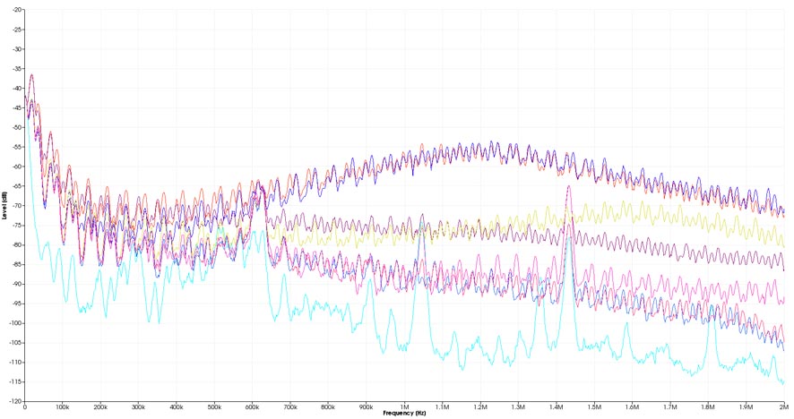
3.2.1. Traces
This visualization is selected as default upon ChipScan-ESA startup. Its properties have been described above.
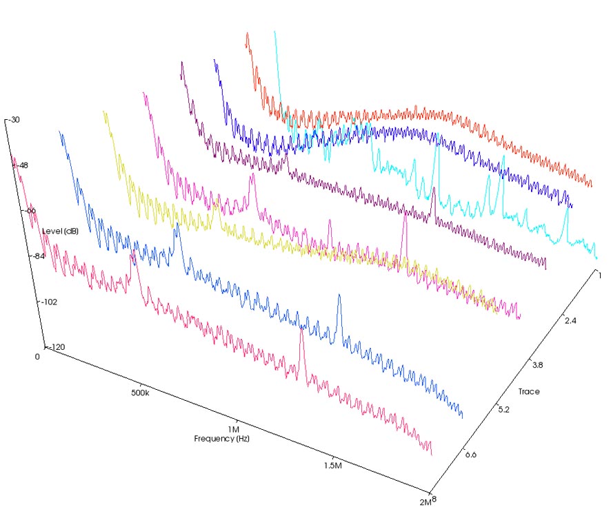
3.2.2. 3D Traces
This visualization displays the traces currently activated in the trace manager one after another in 3D.
3.2.3. Frequency Cut
In this visualization all the traces currently activated in the trace manager are cut at the adjustable frequency and the resulting level values are displayed.
3.3. Spectrum analyzer manager
3.3.1. Spectrum analyzer setup
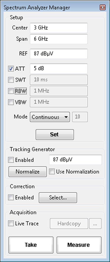
The spectrum analyzer manager lets you set all important properties of your connected spectrum analyzer (see fig 3.5 ). Before using it make sure you properly connected a spectrum analyzer to your PC and have it identified using the device manager. 1 In the following all properties are explained in detail. Keep in mind that none of the properties are transfered to your spectrum analyzer unless you press the Set button. Additionally, changes to properties done via the user interface of the spectrum analyzer are not transfered to ChipScan-ESA. Therefore assume that the properties in the ChipScan-ESA user interface and in the spectrum analyzer may be out of sync.
Frequency range: You can define the frequency range of measured traces by setting a center frequency and a span. Alternatively you can also define the range using a start and a stop frequency. To switch to this mode you need to select Frequency: Start/Stop from the Settings menu.
Reference level: You can set the reference level of the spectrum analyzer. The level can be defined either in dBm or in dBµV. To switch between the units use the Unit entry in the Settings menu. Attenuation: You can either manually set the attenuation of your spectrum analyzer in dB or let the spectrum analyzer set it automatically. The latter is achieved by unchecking the box of the ATT field.
Sweep time: You can either manually set the sweep time of your spectrum analyzer in seconds or let the spectrum analyzer set it automatically. The latter is achieved by unchecking the box of the SWT field.
Resolution bandwidth: You can either manually set the resolution bandwidth of your spectrum analyzer in Hz or let the spectrum analyzer set it automatically. The latter is achieved by unchecking the box of the RBW field.
Video bandwidth: You can either manually set the video bandwidth of your spectrum analyzer in Hz or let the spectrum analyzer set it automatically. The latter is achieved by unchecking the box of the VBW field.
Mode: You can switch between the following modes of your spectrum analyzer: Continuous, Single, Average, Minimum Hold and Maximum Hold. If you selected the Average mode you must also define the number of traces to use to generate the average. Please see the manual of your spectrum analyzer for any details about these modes.
If you have finished to set all properties you must press the Set button to finally transfer the properties to your spectrum analyzer. Furthermore you can set the dB per division value of your spectrum analyzer using the dB/Division entry in the Settingsmenu. To reset your spectrum analyzer to the default settings use the Preset entry in the very same menu.
For reasons of convenience you can also store all properties for future use in a file. To do this use the Save Settings... and Load Settings... entries in the Settings menu. After loading old properties make sure to press the Set button to transfer themto your spectrum analyzer.
3.3.2. Spectrum analyzer normalization
Additionally to setting properties ChipScan-ESA enables you to normalize your spectrum analyzer. This option is only available if your spectrum analyzer includes a supported tracking generator.
To normalize your spectrum analyzer you first need to set the output level of the tracking generator using the appropriate input field. The output level can be defined either in dBm or in dBµV. To switch between the units use the Unit entry in theSettings menu. The second step is to enable the tracking generator by enabling the box to the left of the input field. The last step is to press the Normalize button. Doing this the spectrum analyzer will generate a normalization that is applied to allfollowing measurements. You can also enable or disable the normalization by checking or unchecking the box to the right of the Normalize button.
3.3.3. Trace acquisition and processing
To acquire traces from your spectrum analyzer ChipScan-ESA provides two buttons, Take and Measure. When pressing Take ChipScan-ESA just transfers and displays the trace which is currently located in the spectrum analyzer's memory. When pressing Measure ChipScan-ESA initiates a new measurement in the spectrum analyzer and the resulting trace is displayed in the visualization.
Additionally ChipScan-ESA includes a Live Trace feature. This will continuously transfer the trace from the spectrum analyzer's memory and display it together with all previously acquired traces. You can enable this feature by checking the box Live Trace.
The trace processing in ChipScan-ESA is split into three separate parts. Each of it can be controlled independently.
- Normalization in spectrum analyzer
- Application of correction factors
- Application of mathematical operators
The normalization allows a preprocessing of traces directly within the spectrum analyzer.2
The application of correction factors is the first step in the postprocessing pipeline. In this step all correction factors enabled via the corrections selector dialog will be applied automatically to any acquired traces.3 The corrections selector dialog can be opened by pressing the Select... button in the Correction section of the spectrum analyzer manager. You can turn on or off the application of all enabled corrections by enabling or disabling the box left of the Select... button. A light red dot right of the Select... button indicates enabled correction.
The second step in the postprocessing pipeline is the manual application of mathematical operators via the trace manager. Please have a look at section 3.4 for all details.
3.4. Trace manager
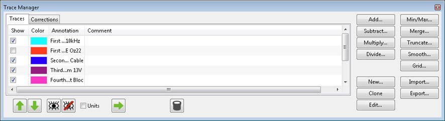
The trace manager holds a list of all available traces and a list of all available corrections. For both lists it shows their properties; visibility, color, x- and y-axis unit, annotation, comments (see fig 3.6. ) and correction categories. As traces and corrections are treated similarly by the trace manager apart from being held in separate lists from now on weonly use the term traces for both of them. Furthermore the trace manager provides all sorts of actions to manipulate the traces. You can either alter the above properties or you can change the data of a trace itself. New traces can be created as well. By selecting the Units checkbox the columns Y Unit and Disp. U. are shown additionally. The former column prints the traces y unit and the latter one prints the currently used unit for the visualization as the visualization can be setup to use a linear or logarithmic y axis and therefore the traces actual y values may be converted accordingly.
3.4.1. Manipulation of trace properties
Trace order: You can change the order of traces in the trace manager by selecting one or more traces and pressing  /
/ . This may be usefull to alter the order of the traces to suit your needs better or to better see parts of traces in the visualization where they overlap.
Visibility: You can alter the visibility of traces in the visualization by selecting or deselecting the box in the Show column of the appropriate line in the trace manager. To show or hide multiple traces you need to select these traces in the trace manager and press .
Color: You can change the color of a trace in the visualization by moving the mouse pointer over the appropriate colored rectangle in the Color column and pressing the left mouse button. In the subsequent color dialog select a new color and click the OK button.
Annotation and comment: To edit the annotation or the comment of a trace first select the appropriate line in the trace manager. Afterwards move the mouse pointer over the annotation or comment column and press the left mouse button. Now you can edit the highlighted string. Please keep in mind that the legend in the visualization displays only the first thirty characters of the annotation.
Correction categories: Corrections are sorted into categories for ease of use. Categories can be enabled or disabled for viewing in the trace manager by the corresponding category checkbox. Newly created corrections get the New category and are visible always. The category of a specific correction can be changed by clicking in the Category column of the selected correction.
3.4.2. Manipulation of trace data
All actions to manipulate trace data are accomplished by pressing one of the buttons on the right of the trace manager. In the following the possible actions are presented.
Addition, subtraction, multiplication, division: Any of these operators can be applied to a number of selected traces. For example if you press the Add... button you can choose between three possibilities. You can add a constant to all selected traces, sum up all traces or add one of the selected traces to all other selected traces. Depending on your selection one or more new traces are generated and are appended to the end of the list of traces.
Min/Max: You can create a maximum or minimum trace from any number of selected traces. Doing so will generate a trace that contains the maximal or minimal value of all traces for each data point.
Merge: The merge operator will merge all of the selected traces into one trace. For example if two traces define two different frequency ranges the resulting trace will contain the data points of both traces. It might happen that multiple traces have overlapping frequency ranges. Therefore when merging the traces an additional dialog is shown whereyou can define the merge order of the traces. The data points of the trace with the highest merge order will be chosen when merging overlapping frequency ranges.
Truncate: You can truncate any number of data points from the start or the end of a trace by defining a new frequency range. Doing so will generate a new trace with all data points lying within the specified frequency range.
Smooth: You can smooth the data of a trace by applying a moving average filter with a specific width. Doing so will generate a new smoothed trace.
Grid: You can change the grid of a trace. This comes in handy for example to make it fit the grid of another trace prior to other mathematical operations like add. Doing so will generate a new trace with the new grid using either linear or spline interpolation depending on the Spline interpolation checkbox.
Clone, delete: You can clone any number of selected traces. This will generate a copy of each of the selected traces in the trace manager. You can also delete any number of traces by pressing the button. This will permanently remove all selected traces from the trace manager.
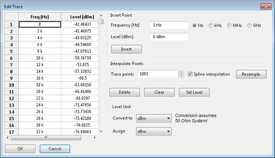
New, edit: You can create a new trace and you can also edit any existing trace. When pressing the appropriate button of either of these operations a subsequent dialog enables you to manage all data points of a specific trace (see fig.3.7 ). You can insert new points by providing an x- and an y-value, you can change the level of all selected points atonce to the level value you provided in the Insert Point section by pressing the Set Level button, you may delete any number of existing points and you may clear all points. You can resample the trace points you inserted so far by entering a number oftarget trace points and pressing the Resample button. If you have enabled the checkbox Spline interpolation the resampling is done using spline interpolation, else linear interpolation is used. Furthermore you can convert the y-values of a trace to a newunit, if there exists a specific conversion. You can also assign a new x- or y-unit to any trace. This will leave the values of the trace unchanged. If you finished all manipulations to data points make sure to press the Ok button to apply all changes. Pressing the Cancel button will abort the operation.
Import, export, copy: You can import traces from ChipScan-ESA files with .csd suffix and corrections from files with .csc suffix by pressing the Import... button. You may also import a single trace from comma separated value list files (.csv) wherein every frequency-value pair has to be on one line starting with the very first line of the file and be seperated by one unique character, e.g. a semi-colon.
You can export selected traces or corrections to ChipScan-ESA files with .csd or .csc suffixes. You may also export as comma separated value list (.csv) for futher statistical analysis with tools like R, Matlab or Excel. Please note that you cannot import .csv files that have been exported from ChipScan-ESA beforehand because the import and export .csv file format differ.
You may copy existing traces from the traces tab to the corrections tab and vise versa, too. To do so select any number of traces from the traces tab or the corrections tab and press the  or the
  button.
3.5. Log
The log collects all additional information on errors, warnings or other output which may occur during the run of ChipScan-ESA. To show the log press Ctrl+L or select the Log entry from the Window menu. While log information is not important forthe user to know it sometimes can be helpful to analyze device communication errors or other complex problems. So if you encounter any problems when running ChipScan-ESA we recommend to read all information in the log before contacting our support. Doingso makes the process of identifying the source of your problem a lot easier. Sometimes we may also ask you to send us all log information to exactly reproduce your problem and eliminate it.
The log collects all additional information on errors, warnings or other output which may occur during the run of ChipScan-ESA. To show the log press Ctrl+L or select the Log entry from the Window menu. While log information is not important for the user to know it sometimes can be helpful to analyze device communication errors or other complex problems. So if you encounter any problems when running ChipScan-ESA we recommend to read all information in the log before contacting our support. Doing so makes the process of identifying the source of your problem a lot easier. Sometimes we may also ask you to send us all log information to exactly reproduce your problem and eliminate it.
4. Managing devices
All devices supported by ChipScan-ESA are managed via the device manager. In general it enables you to detect all connected spectrum analyzers and to select one of them for your subsequent measurements.
4.1. Device detection

Device Interfaces By default only spectrum analyzers connected via GPIB will be detected automatically because it is the most common connection type. If you are using RS232 or LAN/VXI for connection you explicitly need to select the appropriate interface in the device manager to detect your spectrum analyzer. Make sure to disable any unused connection type to shorten the time required for detection. When connecting via RS232 you can additionally provide the specific RS232 port your spectrum analyzer is connected to. This is especially useful to reduce the detection time, if your computer has lots of RS232 ports.1 When connecting via LAN/VXI you must provide the IP address or the appropriate hostname of your spectrum analyzer. Please study your spectrum analyzer manual to gain the required information. If you set all interface properties please press the Detect devices button to identify your devices.
Manual detection In case of detection problems with a device you can also set all connection information manually. To do so please select your spectrum analyzer from the drop down list and set all connection information regarding the interface in the upper part of the device manager. If you set all interface properties please press the Detect Devices button to identify your device.
Last setup Whenever you close the device manager dialog the current device setup will be automatically stored, making it usable for future measurements. So if you open ChipScan-ESA again you can use the last setup to detect your connected devices without setting the interface information. To do this select Load last Setup... in the Devices menu or open the device manager and press the Load last Setup... button.
4.2. Device selection for measurement
If the detection of devices was successful they will be added to drop down lists in the lower part of the device manager. When only one device is found it will be used automatically for the next measurements. When for example multiple spectrum analyzers are found you need to select one of them to be used for subsequent measurements. Keep in mind that you can always switch between multiple devices during your measurements.
4.3. Identifying device communication problems
All drivers for the different supported devices in ChipScan-ESA are intensively tested. If you encounter any problems regarding your device please contact us by writing to software@langer-emv.com. But before contacting us make sure to read the following lines carefully. This may solve your problem right away.
If unable to detect a device When your device can not be detected by ChipScan-ESA first make sure it is included in the list of supported devices (see appendix A). Then check if it is properly connected to the computer. If this is the case please use anysoftware provided by the device manufacturer to make sure the connection between the device and your computer works. If this connection test was successful please deactivate (close) all software that might interfere with the communication between ChipScan-ESA and your device. Especially device manufacturer software for device control or software for logging the communication over the interface are sources for errors. You may also try to perform a manual detection of your device using the device manager.
On errors during measurement If the error only occurs once please repeat your measurement. If the error occurs sporadically or continuously please deactivate (close) all software that might interfere with the communication between ChipScan-ESA and your device. If the error persists please close and reopen ChipScan-ESA. It might also help to restart your computer.
A. Supported spectrum analyzers
The following lists contain all spectrum analyzers supported by ChipScan-ESA, the appropriate supported interfaces (RS232, GPIB1, Ethernet), the firmware version and additional important notes regarding the specific model. If you do not find your spectrum analyzer in the list please contact our sales team for available options using the following email address mail@langer-emv.com.
We are making great efforts to develop our drivers and testing them intensively. Due to different available firmwares for specific spectrum analyzer models we can not guarantee to 100 percent that all spectrum analyzers in these lists are working without any errors. Meaning of icons are:  driver fully tested,
  driver in test phase.
| Advantest | |||||
|---|---|---|---|---|---|
| Model | RS232 | GPIB | Ethernet | Firmware | Notes |
| R3131 | | ||||
| R3131A | | ||||
| R3132 | | | |||
| R3272 | | no hardcopy | |||
| U3741 | | ||||
| U3751 | | ||||
| U3771 | | ||||
| U3772 | | ||||
| Agilent | |||||
|---|---|---|---|---|---|
| Model | RS232 | GPIB | Ethernet | Firmware | Notes |
| E4401B | | | ESA-E series | ||
| E4402B | | | ESA-E series | ||
| E4403B | | | ESA-L series | ||
| E4404B | | | A.07.05 | ESA-E series | |
| E4405B | | | ESA-E series | ||
| E4407B | | | ESA-E series | ||
| E4408B | | | ESA-L series | ||
| E4411B | | | ESA-L series | ||
| E7401A | | | A.02.00 | EMC series | |
| E7402A | | | EMC series | ||
| E7403A | | | EMC series | ||
| E7404A | | | EMC series | ||
| E7405A | | | A.14.04 | EMC series | |
| N9000A | | | A.07.06 | CXA series | |
| N9010A | | | A.14.06 | EXA series | |
| N9020A | | | A.10.52 | MXA series | |
| N9030A | | | A.07.04 | PXA series | |
| N9320B | | 0B.03.43 | no hardcopy, no preset, nouncal | ||
| Hameg | |||||
|---|---|---|---|---|---|
| Model | RS232 | GPIB | Ethernet | Firmware | Notes |
| HM5014 | | ||||
| HM5014-2 | | ||||
| HM5530 | | ||||
| Rigol | |||||
|---|---|---|---|---|---|
| Model | RS232 | GPIB | Ethernet | Firmware | Notes |
| DSA815 | | 00.01.08.00.03 | slow data aquisition | ||
| Rohde & Schwarz | |||||
|---|---|---|---|---|---|
| Model | RS232 | GPIB | Ethernet | Firmware | Notes |
| ESL3 | | 1.83 SP4 | |||
| ESL6 | | ||||
| ESPI3 | | no tracking generator yet | |||
| ESPI7 | | 4.42 | no tracking generator yet | ||
| ESR3 | | | no tracking generator yet | ||
| ESR7 | | | 2.27 SP1 | no tracking generator yet | |
| ESR26 | | | no tracking generator yet | ||
| ESRP3 | | | no tracking generator yet | ||
| ESRP7 | | | 2.26 | no tracking generator yet | |
| ESU8 | | | | 4.43 | hardcopy via GPIB only, no tracking generator yet |
| ESU26 | | | | hardcopy via GPIB only, no tracking generator yet | |
| ESU40 | | | | hardcopy via GPIB only, no tracking generator yet | |
| ETL3 | | | 1.73 | ||
| FSH3 | | several issues | |||
| FSH4 | | no tracking generator | |||
| FSH6 | | V07.11 | several issues | ||
| FSH8 | | V2.50 | no tracking generator | ||
| FSH13 | | no tracking generator | |||
| FSH18 | | several issues | |||
| FSH20 | | no tracking generator | |||
| FSL3 | | | 2.00 SP2 | ||
| FSL6 | | | 1.80 SP1 | ||
| FSL18 | | | 1.80 SP1 | ||
| FSP3 | | | |||
| FSP7 | | | 4.50 | ||
| FSP13 | | | 2.80 | ||
| FSP30 | | | |||
| FSP31 | | | |||
| FSP40 | | | |||
| FSU3 | | | no tracking generator yet | ||
| FSU8 | | | no tracking generator yet | ||
| FSU26 | | | 4.37 | no tracking generator yet | |
| FSU31 | | | no tracking generator yet | ||
| FSU32 | | | no tracking generator yet | ||
| FSU43 | | | no tracking generator yet | ||
| FSU46 | | | no tracking generator yet | ||
| FSU50 | | | no tracking generator yet | ||
| FSU67 | | | no tracking generator yet | ||
| FSUP8 | | | |||
| FSUP26 | | | 4.37 | ||
| FSUP50 | | | |||
| FSV3 | | | 1.50 | ||
| FSV7 | | | |||
| FSV13 | | | 1.50 | ||
| FSV30 | | | |||
| FSV40 | | | |||
| RTO1002 | | 2.70.1.0 | FFT on MATH1 channel | ||
| RTO1004 | | FFT on MATH1 channel | |||
| RTO1012 | | FFT on MATH1 channel | |||
| RTO1014 | | FFT on MATH1 channel | |||
| RTO1022 | | FFT on MATH1 channel | |||
| RTO1024 | | 2.40.1.1 | FFT on MATH1 channel | ||
| RTO1044 | | 2.52.1.1,2.80.1.2 | FFT on MATH1 channel | ||
| Advantest | |||||
|---|---|---|---|---|---|
| Model | RS232 | GPIB | Ethernet | Firmware | Notes |
| RSA6106A | | | no hardcopy | ||
| RSA6114A | | | FV:2.1.0098 | no hardcopy | |
| RSA6120A | | | no hardcopy | ||
Downloads
ChipScan-ESA 3.1.7 - Supported Spectrum Analyzers
To get a demo version of our software for free, please contact our sales team: sales@langer-emv.de